

Quantum Computing
Introduction to Quantum Computing.
First steps in the Quantum Computing world
A series dedicated to those who are taking the first steps in the world of Quantum Computing begins with this article. We begin by clarifying some basic concepts and then we will go into more depth on quantum programming in a friendly way: we will use Hello Quantum, a game made by IBM (it’s an iOS and Android app for your smartphone) to explain how qubits and quantum gates work.
Starting from scratch
Before we deal with quantum computers, what are normal computers?
Put simply, they are devices that store and process information using bits. These are simple chunks of information that take on one of two possible values. We could call these values true and false, or Yes and No, or On and Off, but we usually call them 0 and 1.
Quantum computers instead use qubits. These are quantum objects that can be made to give us a bit. When they are still quantum, we can play with them in ways that are impossible with classical bits. This can can make them harder to keep track of, which is exactly why normal computers struggle to simulate them. But if we know what we are doing, we can harness them to solve problems that even supercomputers couldn’t manage within our lifetime.
Asking qubits questions
The process of obtaining a bit from a qubit is essentially like asking a question. We can ask any of an infinite set of possible questions, each of which can be answered with a simple 0 or 1. Over the last few decades of studying qubits, two possible questions have in particular emerged. So, despite our infinite set of choices, we usually just pick one of these. The way we phrase our questions depends on the way we are describing the qubit. In this article, and in the game Hello Quantum we describe them in a visual way, using a pair of coloured circles.

dotQuantum.io | Quantum Computer Guide Fig 1
One of our questions is to ask about the bottom circle. Is it black, or is it white?
The other question is to ask the same thing about the top one.
Asking qubits questions used to be something only scientists could do. Now anyone can have a go, using the IBM Quantum Experience.
dotQuantum.io | Quantum Computer Guide Fig 2
The IBM Q Experience presents quantum programs using a collection of lines, each of which represents the life of a particular qubit. The events in the life of a qubit are represented by the symbols that are placed on the lines. To ask a question, you just need the right symbols.
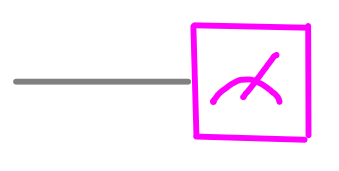
Here is the one you need to ask about the qubit’s bottom circle:
dotQuantum.io | Quantum Computer Guide Fig 3
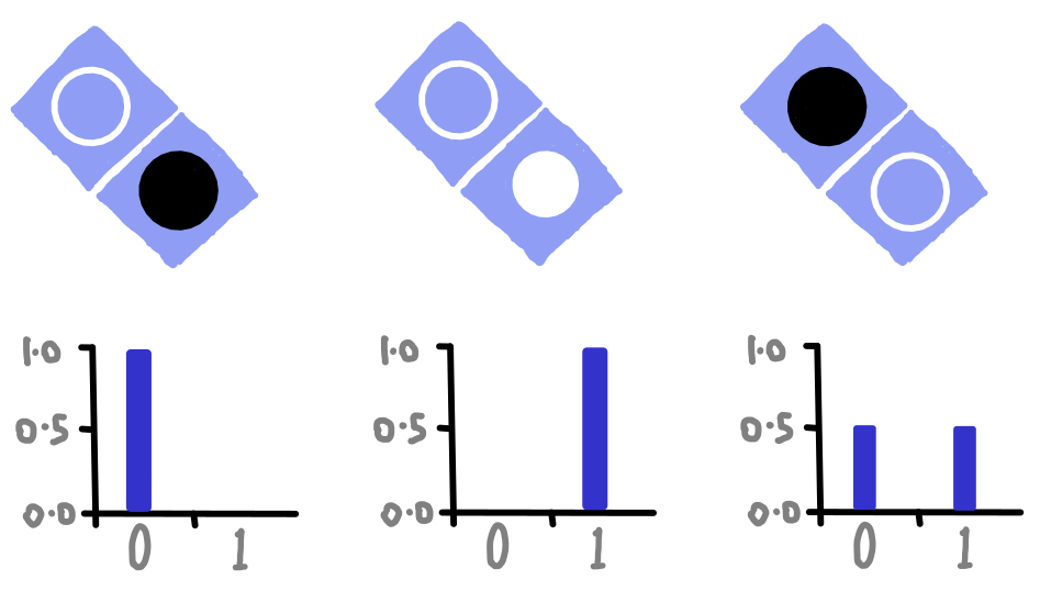
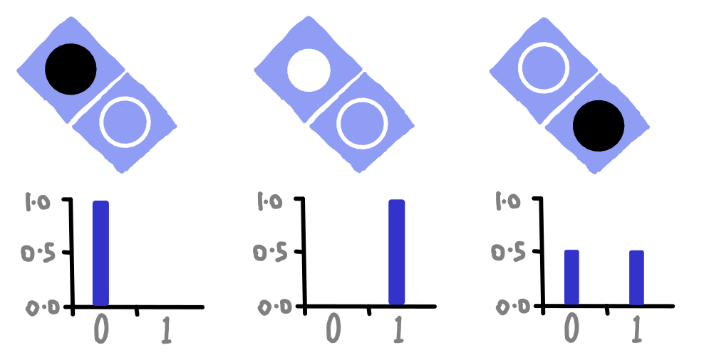
Since we are asking whether the bottom circle is black or white, the bit values we obtain as an answer will reflect these possibilities. We obtain a result of 0 if the bottom circle is black, and 1 if it is white. If it is neither, the qubit is in a bit of a quandry. It can only answer questions with an 0 or 1, because it has no other answer to give. So in the case of an outline circle, it just randomly decides whether to give us an 0 or 1.
dotQuantum.io | Quantum Computer Guide Fig 4
To ask about the top circle, we need to use a couple of symbols (which are called quantum gates, by the way).
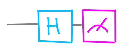
dotQuantum.io | Quantum Computer Guide Fig 5
Asking this question will also result in an answer of 0 or 1, depending on whether the circle is black or white, but it is now the top circle that we are looking at.
dotQuantum.io | Quantum Computer Guide Fig 6
You might have noticed something in the images above. When the top circle is certain of the answer it will give, the bottom one is completely uncertain. And vice versa.
This is because a qubit can only be certain of its answer to one question at a time. This is due to a fundamental uncertainty that exists within quantum systems. The qubit doesn’t really know how it will answer some questions, and only makes up its mind at the moment it is asked the question.
For now, we have only worked with one qubit, but in the next part we will start working on experiments using two qubits.
Adding a second qubit
In the last part, we just talked about one qubit. Now let’s play with two at once. We’ll represent the second qubit in a similar way to the first: as a rectangle containing two circles.
dotQuantum.io | Quantum Computer Guide P2 – Fig 1
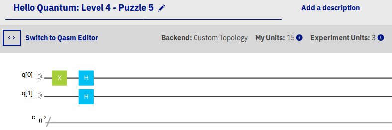
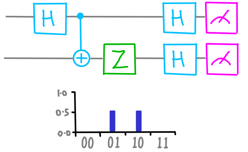
Because of the constantly present randomness, this description isn’t sufficient. For example, here’s something we can do with a couple of qubits before they are measured.
dotQuantum.io | Quantum Computer Guide P2 – Fig 2
This is a small quantum program for two qubits. We’ll get around to explaining all these components later on in this section. But for the moment, just accepted it!
After having run this program, we can ask both qubits about their bottom circles:
dotQuantum.io | Quantum Computer Guide P2 – Fig 3
The results are random. So perhaps all the certainty is in the top circles?
dotQuantum.io | Quantum Computer Guide P2 – Fig 4
No! They are random, too. Our qubits apparently all have outline circles.
dotQuantum.io | Quantum Computer Guide P2 – Fig 5
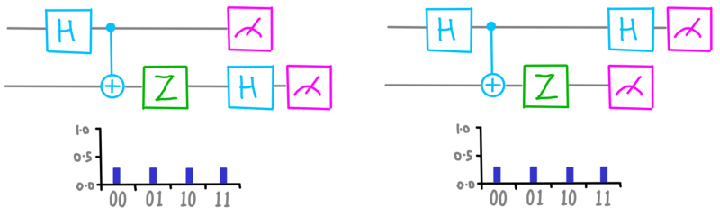
Where has the certainty gone? To find out, try asking the questions at the same time:
dotQuantum.io | Quantum Computer Guide P2 – Fig 6
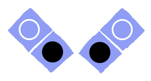
Though both bottom circles give random answers, those answers are certain to be in agreement. This is where our certainty has gone!
This is a rather strange thing to happen. The qubits did not know how they would answer these questions until we asked them. But somehow, they conspired to always agree.
Accounting for effects like this is going to require some extra detail in our visualization of the qubit states. We need to keep track of whether the answers given by the two qubits agree or disagree. And we need to do this for all the possible pairs of questions, whether the answers seem random or not.
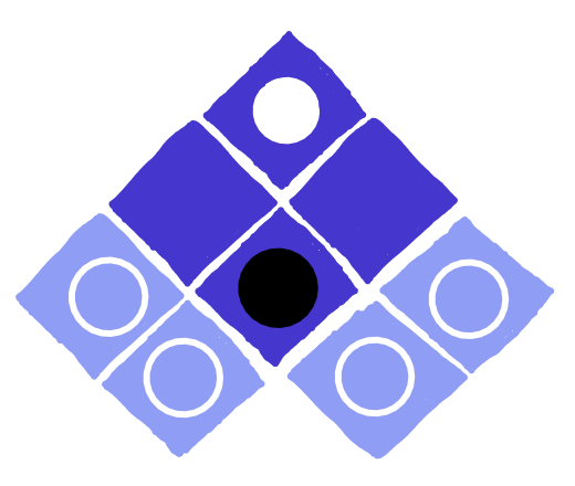
Let’s start by adding another circle, nestled between the bottom ones for the two qubits. When we colour this black, it means that the bottom circles are certain to agree.
dotQuantum.io | Quantum Computer Guide P2 – Fig 7
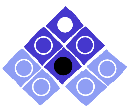
Now, try asking both qubits about their top circle. You’ll find they are certain to disagree.
dotQuantum.io | Quantum Computer Guide P2 – Fig 8
We’ll need to add another circle to represent this. Let’s think of the image as a grid, and put the extra circle where the top rows meet. We’ll represent the certain disagreement by colouring this circle white.
dotQuantum.io | Quantum Computer Guide P2 – Fig 9
We could also ask one qubit about its top circle and the other about its bottom circle. If you try these combinations of measurements, you’ll find that they are equally likely to agree or disagree.
dotQuantum.io | Quantum Computer Guide P2 – Fig 10
This information also needs to be added to our picture. Another couple of circles are needed to fill in the blank spaces. To represent the fact that the agreement (or disagreement) is random, we’ll use outline circles.
dotQuantum.io | Quantum Computer Guide P2 – Fig 11
Now we have a picture that gives us a full description of the answers we expect, whatever questions we choose to ask.
Giving qubits answers
Qubits all start off their life in the same way: when asked about their bottom circle, they’ll give the answer 0. This is called the |0⟩ state.
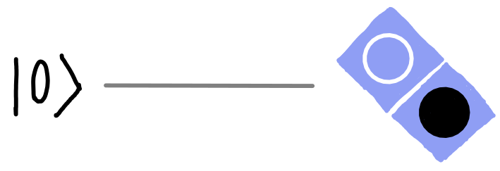
dotQuantum.io | Quantum Computer Guide P2 – Fig 12
So two qubits at the beginning of their lives will look like this:
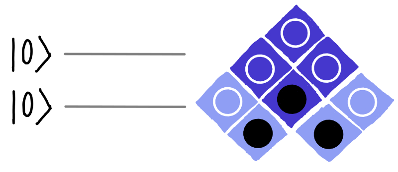
dotQuantum.io | Quantum Computer Guide P2 – Fig 13
When you look at |0⟩, you probably wonder about the | and ⟩. This is called the Dirac notation, but there’s no need to worry about it too much. These notations are basically there as labels, to remind us that this is not the number 0, or a value 0 of the bit, but instead a description of a qubit. We could equally have flagged this by colouring the 0 green, or drawing it on the crown of a princess! Feel free to use whatever convention you prefer.
If our qubits stayed at |0⟩ forever, our quantum computer would be pretty boring. So we need to do something with them. The simplest thing to do is to flip the bottom circle from black to white, or back again. Just like turning on and turning off a light switch. This is done with the X gate.
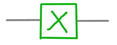
dotQuantum.io | Quantum Computer Guide P2 – Fig 14
Doing this to a qubit flips its bottom circle. So if it was going to answer 0, it will now answer 1, and vice versa. This means obtaining a bottom circle that is white. This is called state |1⟩.

dotQuantum.io | Quantum Computer Guide P2 – Fig 15
Applying an X to an outline circle won’t affect it, because the random state remains random.
Changing the bottom circle of a qubit also affects how it is related to other qubits. Agreements become disagreements, and vice versa. So the effect of X will be to flip a whole row of circles.
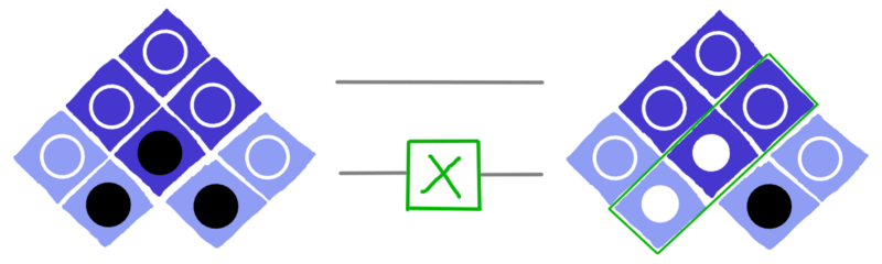
dotQuantum.io | Quantum Computer Guide P2 – Fig 16
In the image above, the X gate is placed on the bottom line, since this corresponds to the qubit on the left of our image. To apply an X to the other qubit, we drag the X gate over to the top line.
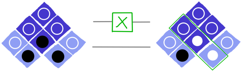
dotQuantum.io | Quantum Computer Guide P2 – Fig 17
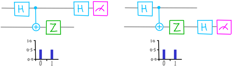
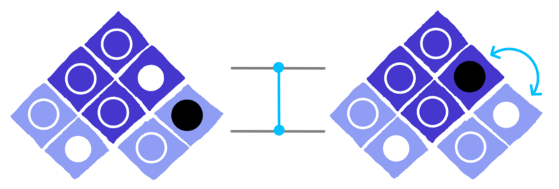
Sometimes we might also want to flip the top circle of a qubit. This is done using a gate called Z. Here is it applied to the qubit on the left.
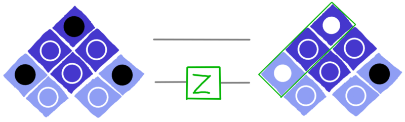
dotQuantum.io | Quantum Computer Guide P2 – Fig 18
These operations, X and Z, are examples of Clifford operations. This fancy name just tells us that they are operations with a relatively straightforward effect on the circles. In fact, this visualization arises from the way we like to think about Clifford operations and their effects.
There are other Clifford operations, too. There is H, which swaps the two circles of a qubit, as well as their corresponding rows:
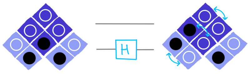
dotQuantum.io | Quantum Computer Guide P2 – Fig 19
With this we can change the questions the qubits have a certain answer to. For example, we can take the state |0⟩ , for which the bottom circle is black, and use the H gate to move that black circle to the top. Then a qubit that was certain to answer 0 when asked about its bottom circle now does so for the top.
The resulting state can’t be |0⟩, because that name has already been taken. So we call it |+⟩.
dotQuantum.io | Quantum Computer Guide P2 – Fig 20
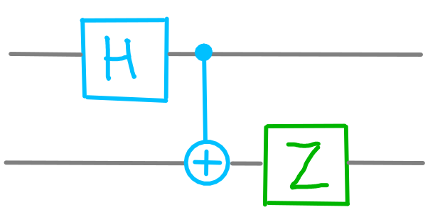
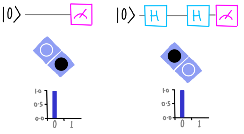
If we apply an X before the H, or a Z after it, we can make its top circle white. This is a state we call |-⟩.
These simple manipulations won’t help us do very much. If we want to use the full potential of quantum computers, we need to use gates that act on both qubits at the same time. We will see this in the next part.
Making qubits talk to each other
As we’ve seen, qubits only have a limited amount of certainty in their answers to questions. When programming quantum computers, our goal is to manage that certainty as best we can. We must guide it on a journey from input to output.
So far, we haven’t got many tools to help us to that. In fact, the H gate is the only one that has moved the certainty around at all. It is hardly enough to explore the entire grid, as you will see by playing levels 1 and 2 of Hello Quantum.
To really get things moving, we need a new kind of gate. We need gates that act on more than one qubit at once. We need controlled gates.
One of the most important controlled operations is the the controlled-Z, also known as the CZ gate. This is the one we introduce in level 3 of Hello Quantum. This is not yet available on the IBM Quantum Experience as a native gate. But if it were, it would look like this:
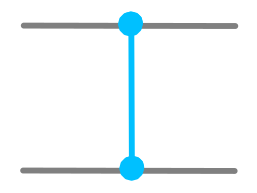
dotQuantum.io | Quantum Computer Guide P2 – Fig 1
There are a few possible ways we can explain the effects of the CZ. Each of these stories seem to be saying something quite different. But somehow, they are all equally true.
One is to say that the CZ first looks at the bottom circle of the left qubit. Depending of whether this circle is white or black, the CZ either does a Z to the right qubit, or does nothing to it. The left qubit is therefore effectively acting like a switch, deciding whether the right qubit gets a Z or not.
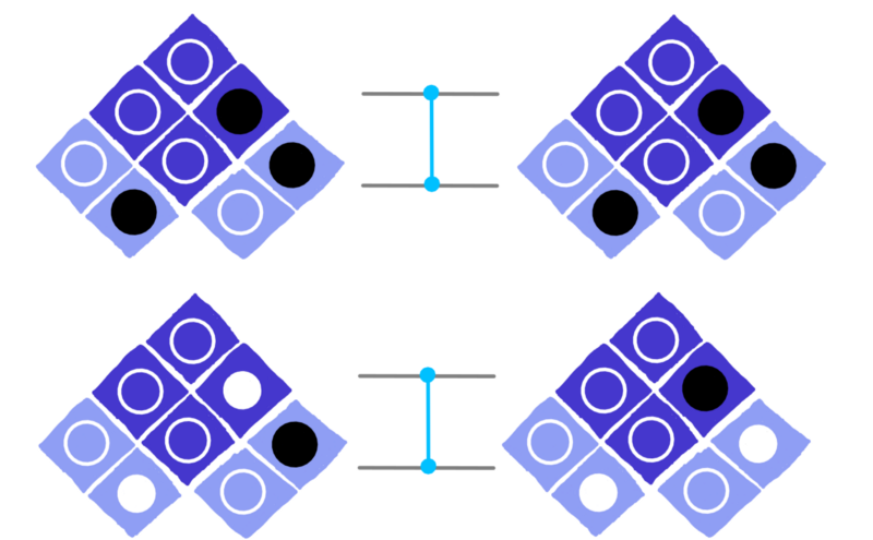
dotQuantum.io | Quantum Computer Guide P2 – Fig 2
Another explanation of the CZ is exactly the same as this, but with the roles of the two qubits reversed.
dotQuantum.io | Quantum Computer Guide P2 – Fig 3
In these examples, it is the right qubit that acts like a switch and the left one that might get a Z. Though it is the exact same CZ, it can be interpreted in the completely opposite way!
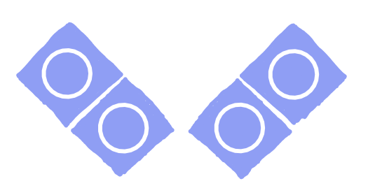
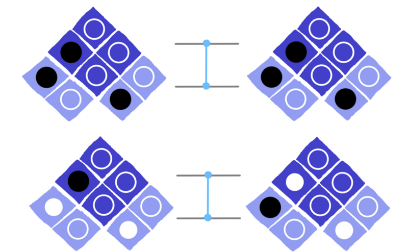
The third way of explaining the CZ is quite different. We can think of it as simply something that moves circles around. Specifically, it swaps two pairs of circles. One pair on the left:
dotQuantum.io | Quantum Computer Guide P2 – Fig 4
And another pair on the right:
dotQuantum.io | Quantum Computer Guide P2 – Fig 5
Though this interpretation is fundamentally different from the other two, it still completely captures the effects of the CZ. You can look at the same CZ acting on the same state, and interpret in any of the three ways.
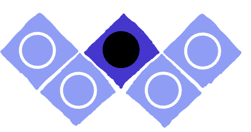
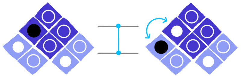
This explanation is not without its troublesome parts. Check out what it does to the circle at the very top of the grid.
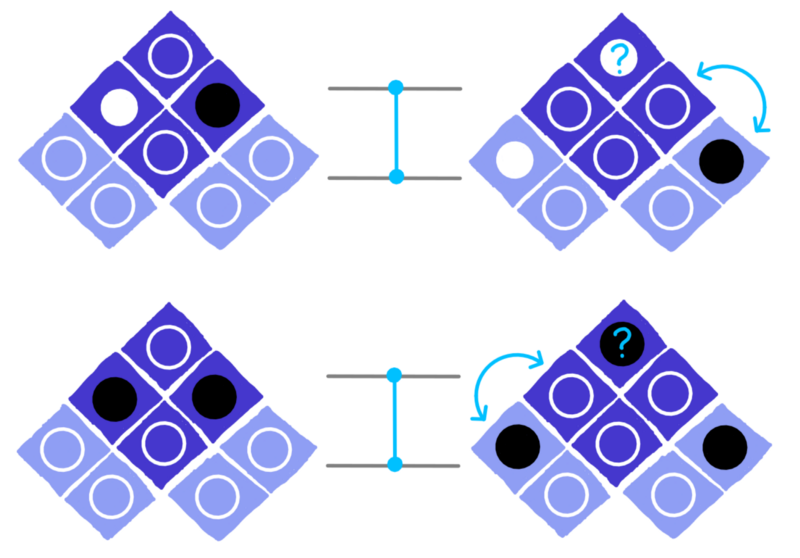
dotQuantum.io | Quantum Computer Guide P2 – Fig 6
In the first example, the circle at the very top was turned from outline to white. In the second, it turned from outline to black. What is the logic behind this?
It’s possible to solve all the puzzles of Hello Quantum without understanding this effect. But if you want to become a quantum programmer, you’d probably like to know what is going on. So we are going to give you the opportunity to find out for yourself!
The only reason this effect doesn’t seem to make much sense is that the grid is not quite big enough. The eight circles don’t fully describe a pair of qubits. For a complete description, we need to add another possible question. On the IBM Quantum Experience, this question can be done with the following gates:
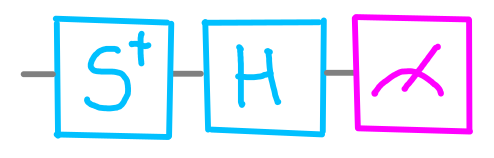
dotQuantum.io | Quantum Computer Guide P2 – Fig 7
To keep track of what answers it will give, we need to add another circle to our description of each qubit.

dotQuantum.io | Quantum Computer Guide P2 – Fig 8
Here the new circle is in the middle, and has been coloured a bit differently to highlight it.
To describe the possible outcomes of the middle circle, and all their possible agreements and disagreements with each other and the other questions, we need a grid with 15 circles.
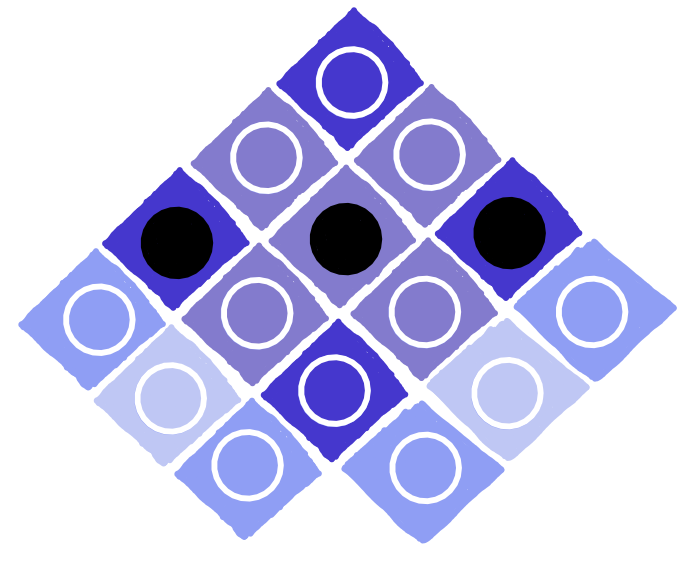
dotQuantum.io | Quantum Computer Guide P2 – Fig 9
With these, you can solve the mystery of the CZ. And you can also check out how the X, Z and H gates affect these new circles, as well as trying out new gates like S. Just get playing with the new measurement on the IBM Quantum Experience, and use your results to understand the bigger grid. We will see how to set up the IBM Q Experience for this in a tutorial that we will publish very soon.
Beyond Clifford
All the gates we’ve discussed so far are what we call Clifford gates. Each can be interpreted in terms of just swapping circles, or flipping them between black and white.
There is much we can do with Clifford gates. They are key to the way we move information around in quantum computers. They are also excellent at error correction, since they can be used to seek out imperfections, tell us where they are, and let is correct them.
For full quantum computation, however, we need something more. We need to move beyond circles that are just black, white or outline. We need to get ones that are ‘mostly black’ or ‘pretty much random, but a bit biased towards white’. We need to spread out the certainty, rather than keeping in little islands. Then after swishing it around the grid for a bit, we can recombine it in new and unexpected ways.
To do these things, we need the unimaginatively named non-Clifford gates.
There are none of these in the app version of Hello Quantum, but there is one in its sister game: a command line version. This has an extra gate called Q for you to try.
dotQuantum.io | Quantum Computing Guide P4 – Hello Quantum Console
Also, the IBM Quantum Experience has a whole host of non-Clifford gates. The easiest ones to try are T and Tdg. You’ll need the full 15 qubit grid to figure these out, but you have all you need to have a go.
Beyond two qubits
The game Hello Quantum helps you build up intuition and knowledge with just two qubits. Once you have that, you can begin tackling larger numbers.
To fully describe three qubits, we’ll again need to keep track of each of how it would answer the three questions. And we’d need to keep track of how answers to questions on one qubit agree or disagree with the others. And how does this relate to what the third one is doing? This needs a lot of circles. A cube full of 63 of them, to be exact.
Extend this to four qubits, and you need a hypercube of 255 circles. For n qubits, it takes 4ⁿ-1. The amount of information we’d need to keep track of increases exponentially with the number of qubits!
This means that visualizations like the one used in Hello Quantum will only ever be useful for small numbers of qubits. After all, if we could visualize what was going on in a large quantum computer easily, it would mean that we can easily simulate it. And if we could easily simulate quantum computers, there’d be no need to build them.
But there is a need to build them. By guiding information through this massive space of possibilities, we can find routes from input to output that would be impossible on a standard computer. Sometimes, these will be a lot faster. Some programs that would take a planet sized supercomputer the age of the universe to solve will be doable with much more reasonably sized quantum computers in a much more reasonable time.
Getting to know a quantum processor
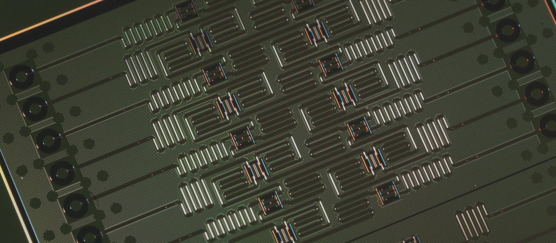
Quantum computers are built out of qubits. But just having lots of qubits is not enough. A billion qubits working in complete isolation will never achieve anything. They need to talk to each other. This means that the need to be connected by so-called controlled operations. Every device has its own rules for which pairs of qubits can be connected in this way. The better the connectivity of a device, the faster and easier it will be for us to implement powerful quantum algorithms.
The nature of errors is also an important factor. In the near-term era of quantum computing, nothing will be quite perfect. So we need to know what kinds of errors will happen, how likely they are, and whether it is possible to mitigate their effects in the applications we care about.
These are the three most important aspects of a quantum device: qubit number, connectivity and noise level. To have any idea of what a quantum computer can do, you need to know them all.
So let’s make a game that runs on a quantum device and shows all these things directly. By just playing the game, the player will see exactly how big and connected the device is. By comparing a run on the real device with one on a simulator, they’ll see exactly how potent the noise is. Then by playing again with some error mitigation, they’ll get an idea of how much useful information can be salvaged even in the era of slightly noisy quantum computers. We’ll call this game Quantum Awesomeness, and we’ll play it on the IBM device known as ibmq_16_melbourne.
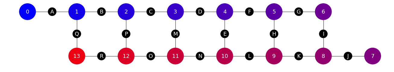
dotQuantum.io | Quantum Computer Guide Quantum Processor – Fig 1
The image above gives a quick guide to what’s going on in the Melbourne device. There are 14 qubits, numbered from 0 to 13, shown by coloured circles. The qubits that can talk to each other via a controlled operation are shown connected by lines, each of which has been given a letter for a name.
The most useful thing you can do with controlled operations is create and manipulate entanglement. Only with this can we explore the full space of possibilities that is open to our qubits, and hope to do things that are practically impossible for classical computers.
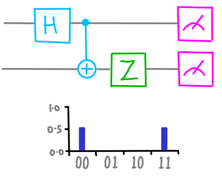
The simplest kind of entanglement involves just two qubits. It will cause each to yield outputs that are random, but with correlations between them. For example, consider following program on a couple of qubits.
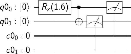
dotQuantum.io | Quantum Computer Guide Quantum Processor – Fig 2
This is a circuit diagram: a history of the qubits in our program told from left to right.
Here we perform an rx operation for the angle π/2, which results in what is essentially half an x gate. This is an example of what we called a ‘partial NOT’ in the Battleships with partial NOT gates game. Instead of flipping the qubit all the way from |0⟩ to |1⟩, it parks it in a quantum superposition state in-between.
The operation acting on both qubits is a controlled-NOT, which applies a NOT to the bottom qubit only when the top one is in state |1⟩. Since the top one is in a superposition of both possibilities, the effect of the controlled-NOT is to spread the superposition to the bottom qubit as well: a combined superposition of both |0⟩ and both |1⟩.
The final part of the circuit is to extract a simple bit from each qubit: |0⟩ becomes 0, |0⟩ becomes 1, and a superposition becomes a random choice of one or the other. But even though both qubits will give a random result in this case, they are sure to always agree.
To verify this, let’s run it. The result I got was,
{'11': 503, '00': 521}
Out of the 1024 samples that the program was run for, all results came out either ‘00’ or ‘11’. And we have approximately equal numbers of samples for each. All as predicted.
By replacing the value of π/2 we can change the nature of the superposition. A lower value will produce results more biased to outputs of 0, and a value closer to π will result in a bias towards 1s. This means we can vary the probability with which each output will give a 1. But whatever value we choose, this form of circuit ensures that the results for the two qubits will always agree.
In this game we will make lots of these pairs of entangled qubits across the device. To do this, we must first choose a way to pair up the qubits monogamously (possibly leaving some spare ones left over). This pairing will be chosen randomly, and the whole point of the game is for the player to guess what the pairing was.
Once we have the random pairing, we’ll basically run the quantum program above on each independent pair. Though we will introduce one difference: for each pair we’ll randomly choose a different value for the rx operation, so the degree of randomness shared by paired qubits will differ from pair to pair.
When we run the circuit, the result will be a string of 14 bits: with each bit describing the output of each qubit. Since we run it for many samples to take statistics, the full result will be a list of all the bit strings that came out, along with the number of times that each occurred.
Since the aim of the game is for the player to deduce the pairing from the output, we could just dump all this data on them. But that probably wouldn’t be very fun. Instead, we can just focus on the important points:
What is the probability of each qubit giving an output of 1 instead of 0?
What is the probability that each pair of connected qubits give the same value?
We can then put that information on our image of the device. For example, here’s one particular set of runs.
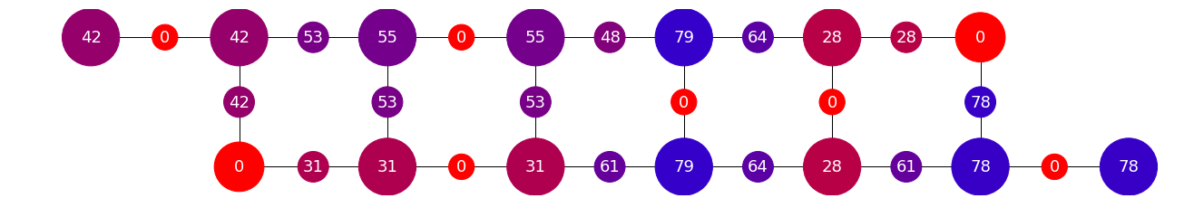
dotQuantum.io | Quantum Computer Guide Quantum Processor – Fig 3
The number displayed on each qubit is the percentage of samples for which the result was 1. The number on each connection is the percentage of samples for which the corresponding pair of qubits had outcomes that disagreed
With this information, we can easily find the pairs of qubits that were entangled: either by looking for the qubits that share the same probability of outputting a 1, or finding the pairs that never disagreed.
The above data was extracted from a simulator. Now let’s try it on the real quantum device.
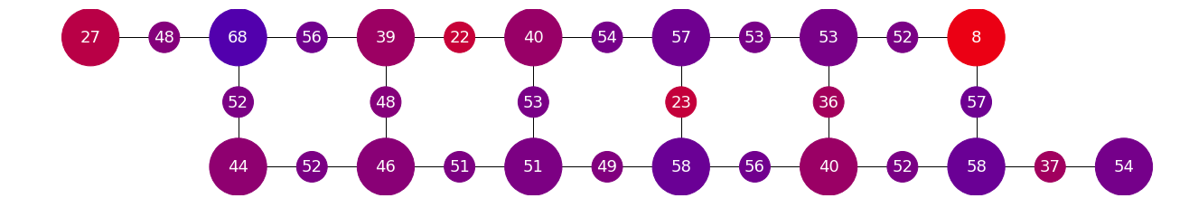
dotQuantum.io | Quantum Computer Guide Quantum Processor – Fig 4
Here the results are not so clear as for the simulator. The effects of noise are much stronger, making it much harder to identify the pairs.
But all is not lost! We can do some error mitigation. We know that the output should have a certain structure, so we can search for that structure and use it to clean up the result.
Here’s a very simplistic way to do that. First, each qubit will look at all its neighbours and see which one it agrees with most. It’ll then assume that this most agreeable qubit is its partner. To try and balance out the errors in its results, we’ll then replace the probability of getting an output of 1 for that qubit with the average from them both.
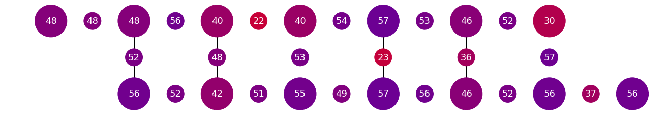
dotQuantum.io | Quantum Computer Guide Quantum Processor – Fig 5
Though things have improved, they’ve not been made perfect by any means. This is because our error mitigation scheme is pretty simple, and is just bolted on at the end of the process. Error mitigation can have powerful effects, but it is most effective when built into the quantum program itself (something you could try to experiment with if yourself if you’d like to expand upon this project).
For now, let’s just play the game using these mitigated results.
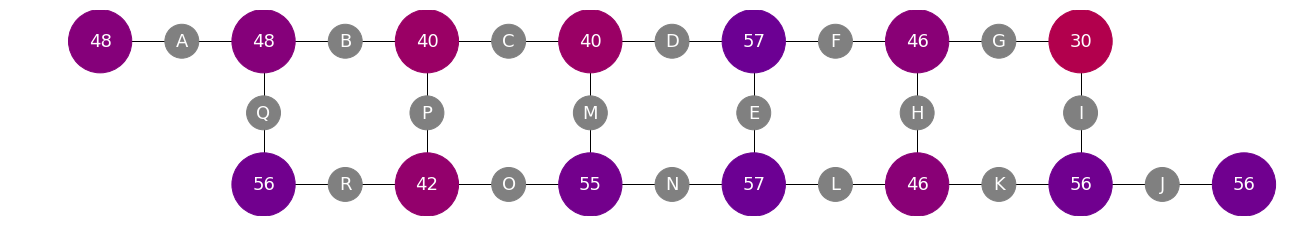
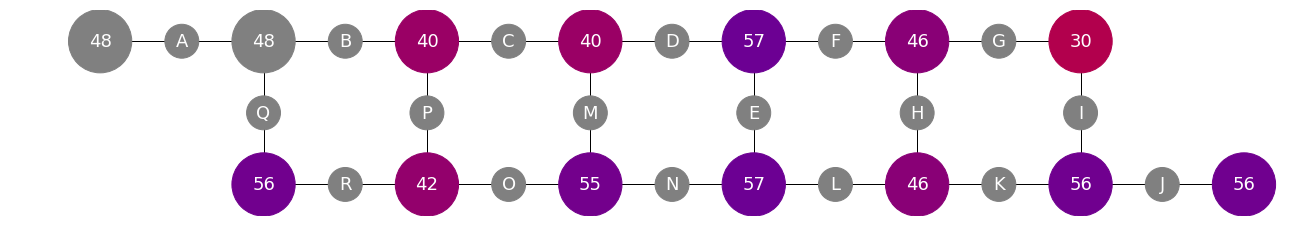
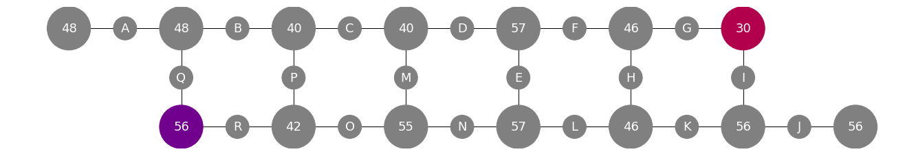
dotQuantum.io | Quantum Computer Guide Quantum Processor – Fig 6
Our job is to look at the numbers on the qubits, and try to find pairs that either have the same number, or at least have numbers that are close as possible. The two 48s on the left seem like a good start. So let’s go for pair A as one we think is entangled.
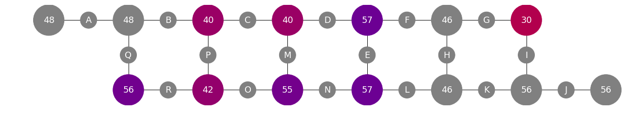
dotQuantum.io | Quantum Computer Guide Quantum Processor – Fig 7
The two 46s of pair H are the same as each other, and also quite distinct from their neighbours. So we’ll go for that one too.
dotQuantum.io | Quantum Computer Guide Quantum Processor – Fig 8
Then pair E seems pretty certain.
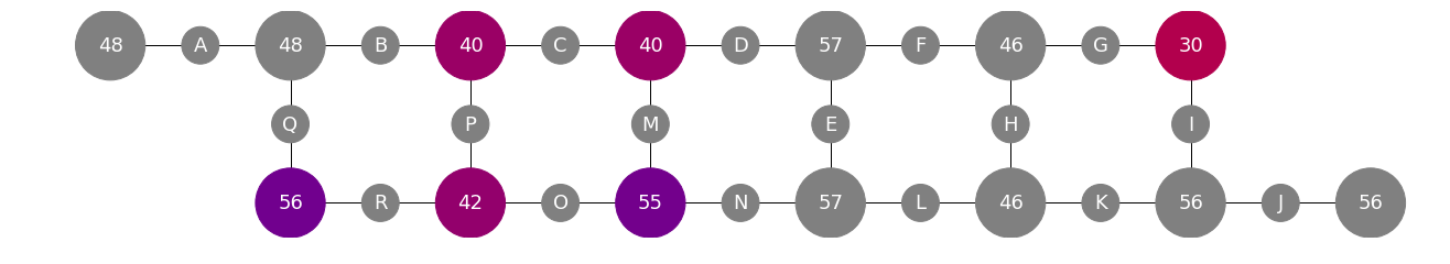
dotQuantum.io | Quantum Computer Guide Quantum Processor – Fig 9
And pair C.
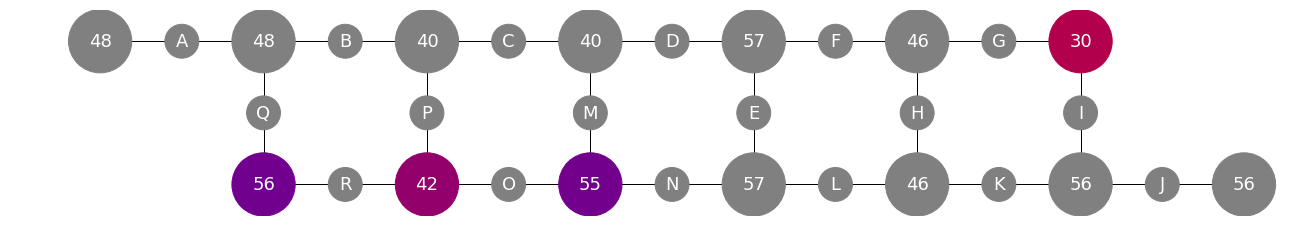
dotQuantum.io | Quantum Computer Guide Quantum Processor – Fig 10
Now we’ve reached a point where noise makes it a little hard for us. Should the 42 be paired with the 55, or the 56? Since the 55 is closer in value, we’ll go for pair O.
dotQuantum.io | Quantum Computer Guide Quantum Processor – Fig 11
Finally we are left with two qubits that must have been paired with nothing. That will always happen on this device due to the way its connectivity graph is structured. So we have reached the solution! But was it the correct one?
Let’s look again at the noiseless simulation, where the correct pairing was much easier to see.

dotQuantum.io | Quantum Computer Guide Quantum Processor – Fig 12
The pairs that show perfect agreement here are exactly the ones we just chose. So we were indeed correct. We played a game on a quantum computer, and we won!If you want to get started with quantum programming, why not take a look at the source code for this game, available on the Qiskit tutorial.
Join dotQuantum
Become Part Of The Future Quantum Bit World!!
By clicking on “SUBSCRIBE” you agree to receive our monthly newsletter (Read the Privacy Policy). You can unsubscribe at any time by clicking on the link in the newsletter that we will send you.